Noise Noise Everywhere
Polynomial regression grapples with noisy data, challenging R-squared values. This article uses Python and techniques like Cook's and Mahalanobis Distance to enhance model reliability.
Objective
In the realm of statistical modeling, polynomial regression often encounters the complexities of dealing with noisy data, which can pose significant challenges. When R-squared values deviate from the expected 1 or -1, it prompts questions about the model's accuracy. In this article, we'll guide you on enhancing the reliability and performance of polynomial regression models, even when faced with noisy data. Our toolkit includes Python and techniques like Cook's and Mahalanobis Distance to address these challenges.
I utilized Python to address the challenge of fitting noisy univariate data into a polynomial regression model. Once the model was constructed, my focus shifted towards uncovering valuable insights regarding the optimal independent variable values that could maximize the dependent variable's performance. To achieve this, I harnessed Python's built-in statsmodels library and employed Ordinary Least Squares (OLS) modeling to effectively fit the parameters into a polynomial equation of degree 2. Subsequently, I calculated the R-squared values for two key parameters: Parameter 1, which exhibited a decreasing trend over time (measured in hours), and Parameter 2, which displayed an increasing trend.
To tackle the challenge of noise interfering with model fitting, I employed two distinct methods:
1. Cook's Distance: I utilized this method to identify and filter data points based on a predefined Cook's distance threshold. This approach is particularly effective for univariate data.
2. Mahalanobis Distance: For multivariate data, I opted for this method, filtering data points based on a Chi-Squared threshold associated with Mahalanobis distance. It is relevant to note that Mahalanobis distance can also be used for univariate data, as it will just change multidimensional matrix of values(in case of multiple features) to a 1-D matrix (in case of one feature).
Background
Before proceeding further, let's delve into Cook's Distance and Mahalanobis Distance a little more.
Cook's Distance measures the influence of each data point on the coefficients of a statistical model, such as linear regression. It helps identify influential data points that have a significant impact on the model's parameters. Greater Cook's distances indicate data points that potentially have a substantial influence on the model and may be considered as outliers or noisy data points.
The formula for Cook's distance for a data point 'i' in a linear regression model is:
Di is Cook's distance for data point i.
ei is the residual (the difference between the observed and predicted values) for data point i.
k is the number of model parameters (including the intercept).
MSE is the mean squared error of the model.
hi is the leverage of data point i, which measures how far the predictor variables for that data point are from the mean predictor values.
To filter noisy data using Cook's Distance, a typical approach is to set a threshold value (e.g., 4 times the mean Cook's Distance or 4/N where N is length of dataset) and consider data points with Cook's Distance greater than this threshold as potential outliers or noisy data.
The Mahalanobis Distance, on the other hand, is used for multivariate data and measures the distance between a data point and the center of the data distribution, taking into account the covariance structure of the data. It is particularly useful for detecting outliers in multivariate datasets.
The formula for Mahalanobis Distance for a data point 'x' with mean vector 'μ' and covariance matrix 'Σ' is:
To filter noisy data using Mahalanobis Distance, we typically calculate the Mahalanobis Distance for each data point and compare it to a threshold. Data points with Mahalanobis Distances greater than the threshold are considered outliers or noisy data points. The threshold can be determined based on a chosen significance level or through methods like the chi-squared distribution.
Method
In the following discussion, I will demonstrate both approaches and illustrate how adjusting the threshold values and filtering noisy data can significantly enhance the robustness of the model without significantly impacting the fitted parameters.
A sample Excel data file that will be used in this analysis is shared below.
Import Relevant Libraries
import statsmodels.api as sm # For OLS fitting of the data
import pandas as pd # For importing, cleaning and organizing data
import numpy as np # For numerical computations
import matplotlib.pyplot as plt # For plotting curves
import scipy as stats
from scipy.stats import chi2 # For calculating mahalanobis threshold
Assign Feature and Target Variables
Assuming 'Parameter 2' (or 'Parameter 1') as the dependent variable and 'Time (Hr)' as the independent variable, I fetched the pandas dataframe (same initial data is used for filtered and unfiltered dataframes) and assigned X and y values as follows:
# Assuming "Parameter 2" as the dependent variable and "Time (Hr)" as the independent variable
data = pd.read_excel('Sample Data.xlsx') # For noisy data plotting
data_cook = pd.read_excel('Sample Data.xlsx') # For Cook's filtering
data_mah = pd.read_excel('Sample Data.xlsx') # For Mahalanobis filtering

X = data[["Time (Hr)"]]
y = data["Parameter 2"]
To gain an initial understanding of the noisy data, I conducted multiple curve fittings using Ordinary Least Squares (OLS) to determine the best-fitting model. In the current context, the model that fits best is a degree-2 polynomial, expressed as follows:
Where βn (n=0,1,2) are the coefficients for the respective degrees corresponding to 'Time (Hr)' independent variable.
Fit OLS Model
We then fitted the OLS model and calculated the R-squared value of the noisy dataset.
# Polynomial Regression (Degree 2)
# Add a dictionay of coefficients from degrees 1 and 2.
# Constant coefficient (degree 0) is inheretied as 'const'

X_poly = sm.add_constant(pd.DataFrame({'Time (Hr)': X['Time (Hr)'], 'Time (Hr)^2': X['Time (Hr)'] ** 2}))
model_poly = sm.OLS(y, X_poly).fit()
r_squared = model_poly.rsquared

# Write the polynomial equation as mentioned before after taking
# the coefficients of degrees 0, 1 and 2 and
# rounding the values to 2 decimal places

equation_poly = "Parameter 2 = {} + {} * Time (Hr) - {} * (Time (Hr))²".format(round(model_poly.params['const'], 2), \                                                                  round(model_poly.params['Time (Hr)'], 2), \                                                                  -round(model_poly.params['Time (Hr)^2'], 2))
Next, we visualized the scatter plot of Parameter 2 versus Time (Hr) along with R-squared values and the polynomial equation.
fig, axes = plt.subplots(1, figsize=(10, 5), gridspec_kw={'hspace': 0.5})

# Plot unfiltered data using scatter plot of
# Time (Hr) versus Parameter 2

axes.scatter(data["Time (Hr)"], data["Parameter 1"], label=f"Initial Data (R-sq: {r_squared:.2f})", alpha=0.5)
axes.set_xlabel("Time (Hr)")
axes.set_ylabel("Parameter 1")
axes.legend(loc=(1.01,0.5))
axes.text(0.1, 0.5, equation_poly, transform=axes.transAxes)  # Display annotation on the current subplot
axes.set_title(f"Unfiltered Data Polynomial Regression")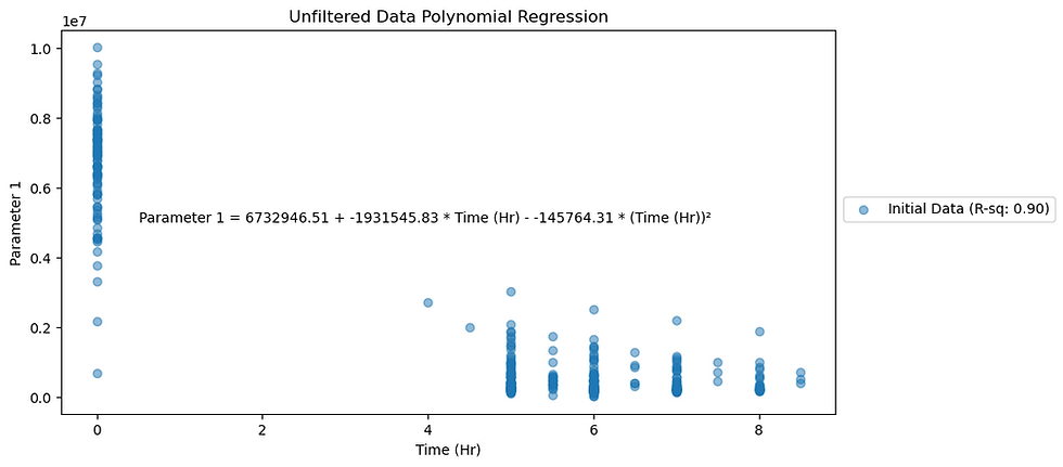
Figure 1. Noisy data plotted for Parameter 1.

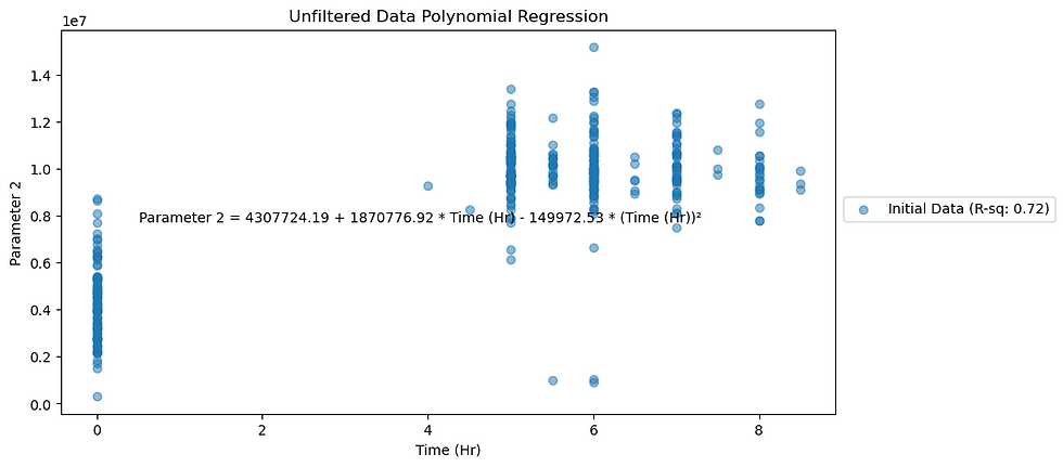
Figure 2. Noisy data plotted for Parameter 2.
Noisy data plots show R-squared values for Parameters 1 and 2 as 0.90 and 0.72 respectively.
Filter Data Using Cook's Distance
I applied both filtering techniques to 'Parameter 1' and 'Parameter 2' and found significant improvements in R-squared values, especially using Cook's Distance.
To calculate the Cook's threshold, I created a list of numbers and divided them by the length of the dataset. I also initiated an empty list to calculate and append R-squared values in filtered datasets.
# Create a list of i values for Cook's threshold
# Where Cook's Threshold is i/N where N is the length of the dataset
cook_threshold_values = [0.1, 0.25, 0.5, 1, 2, 4, 8]
cook_threshold_values.reverse()
r_squared_values_cook = []
Then, I filtered out data points whose values were greater than the Cook's threshold. I plotted the unfiltered data on the same plots as the filtered data, to get a sense of which data points were found to be outliers for a particular Cook's threshold value. Here, it is important to note how we used the get_influence.cooks_distance[0] functionality of the fitted model model_poly to get respective Cook's distances for each data point.
influence_poly = model_poly.get_influence()
cooks_d2_poly = influence_poly.cooks_distance[0]
data_cook['Cooks Distance'] = cooks_d2_poly
Thereafter the Cook's threshold value was calculated for each case.
for i, cook_threshold_value in enumerate(cook_threshold_values):
    # Calculate Cook's distance for each observation in the data
    cook_threshold_poly = cook_threshold_value / len(data_cook)
All those data indices where the Cook's distance was less than the Cook's threshold were then filtered using np.where functionality. These indices were used with .iloc to locate the rows with filtered indices in the pandas dataframe.
    filtered_indices_poly = np.where(cooks_d2_poly <= cook_threshold_poly)[0]
    filtered_data_poly_cook = data.iloc[filtered_indices_poly]
Therafter, a similar OLS model fitting was done on the filtered dataset as mentioned earlier for the unfiltered data.
    X_filtered_poly_cook = filtered_data_poly_cook[["Time (Hr)"]]
    y_filtered_poly_cook = filtered_data_poly_cook["Parameter 2"]
    X_poly_filtered_cook = sm.add_constant(pd.DataFrame({'Time (Hr)': X_filtered_poly_cook['Time (Hr)'], \
                                                         'Time (Hr)^2': X_filtered_poly_cook['Time (Hr)'] ** 2}))
    model_poly_filtered_cook = sm.OLS(y_filtered_poly_cook, X_poly_filtered_cook).fit()

    equation_poly = "Parameter 2 = {} + {} * Time (Hr) - {} * (Time (Hr))²".format(round(model_poly_filtered_cook.params['const'], 2), \                                                                  round(model_poly_filtered_cook.params['Time (Hr)'], 2), \                                                                  -round(model_poly_filtered_cook.params['Time (Hr)^2'], 2))

    r_squared_cook = model_poly_filtered_cook.rsquared
Then, after applying a 'for loop' that filtered the initial dataset for various values of Cook's threshold, I also calculated the R-squared values for each case and plotted them on scatter plots for visualization. Python code for the 'for loop' and the corresponding scatter plots is shown below.
# Create subplots for Cook's distance filtering
fig, axes_cook = plt.subplots(len(cook_threshold_values), figsize=(8, 20), gridspec_kw={'hspace': 0.5})

for i, cook_threshold_value in enumerate(cook_threshold_values):
    cook_threshold_poly = cook_threshold_value / len(data_cook)
    filtered_indices_poly = np.where(cooks_d2_poly <= cook_threshold_poly)[0]
    filtered_data_poly_cook = data_cook.iloc[filtered_indices_poly]
    X_filtered_poly_cook = filtered_data_poly_cook[["Time (Hr)"]]
    y_filtered_poly_cook = filtered_data_poly_cook["Parameter 2"]
    X_poly_filtered_cook = sm.add_constant(pd.DataFrame({'Time (Hr)': X_filtered_poly_cook['Time (Hr)'], \
                                                         'Time (Hr)^2': X_filtered_poly_cook['Time (Hr)'] ** 2}))
    model_poly_filtered_cook = sm.OLS(y_filtered_poly_cook, X_poly_filtered_cook).fit()

    equation_poly = "Parameter 2 = {} + {} * Time (Hr) - {} * (Time (Hr))²".format(round(model_poly_filtered_cook.params['const'], 2), \                                                                  round(model_poly_filtered_cook.params['Time (Hr)'], 2), \                                                                  -round(model_poly_filtered_cook.params['Time (Hr)^2'], 2))

    r_squared_cook = model_poly_filtered_cook.rsquared

    # Plot initial data
    axes_cook[i].scatter(data_cook["Time (Hr)"], data_cook["Parameter 2"], label="Initial Data", alpha=0.5)
    axes_cook[i].scatter(filtered_data_poly_cook["Time (Hr)"], \
                y_filtered_poly_cook, label=f"Filtered Data(R-sq: {r_squared_cook:.2f})", alpha=0.5)
    axes_cook[i].set_xlabel("Time (Hr)")
    axes_cook[i].set_ylabel("Parameter 2")
    axes_cook[i].legend(loc=(1.01,0.5))
    axes_cook[i].text(0.1, 0.1, equation_poly, transform=axes_cook[i].transAxes)  # Display annotation on the current subplot
    axes_cook[i].set_title(f"Cook's Distance Filtering (Threshold = {cook_threshold_value}/N = {cook_threshold_poly:.4f})")
Scatter plots below show the noisy and filtered data along with their respective R-squared values after fitting the OLS model.

Figure 3. Filtered data (by Cook's Distance analysis) plotted for Parameter 1.

Figure 4. Filtered data (by Cook's Distance analysis) plotted for Parameter 2.
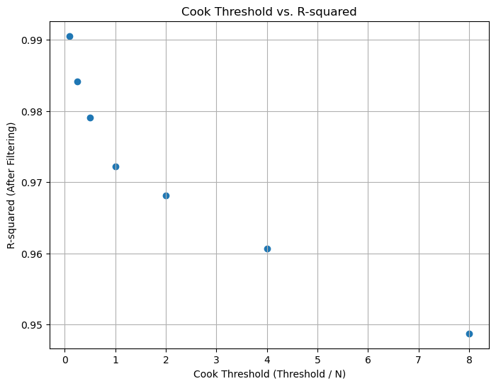
Figure 5. Cook's Threshold vs R-Squared values for Parameter 1.
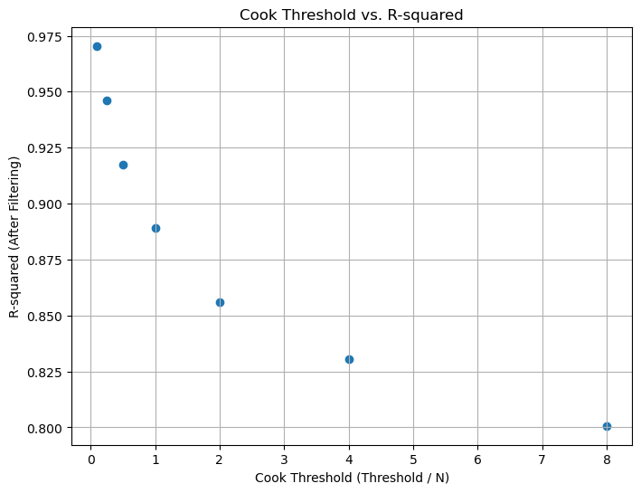
Figure 6. Cook's Threshold vs R-Squared values for Parameter 2.
We can observe that as the Cook's threshold decreases, the R-squared values for the dataset increase, as shown in the plots below. Irrespective of the threshold value chosen, these R-squared values are higher than those of noisy data (0.90 for Parameter 1, 0.72 for Parameter 2). However, there's a trade-off between filtering and information loss, so choosing an optimum Cook's threshold is crucial.
Filtering Data Using Mahalanobis Distance
To calculate the Mahalanobis distance using the formula provided earlier, we apply a calculateMahalanobis function to the dataset as shown below.
def calculateMahalanobis(y=None, data=None, cov=None):

    y_mu = y - np.mean(data)
    if not cov:
        cov = np.cov(data.values.T)
    inv_covmat = np.linalg.inv(cov)
    left = np.dot(y_mu, inv_covmat)
    mahal = np.dot(left, y_mu.T)
    return mahal.diagonal()

data_mah['Mahalanobis']= calculateMahalanobis(y=data_mah, data=data_mah[['Time (Hr)', 'Parameter 1', 'Parameter 2']])
Here, we extensively use numpy matrix calculation functionalities, after subtracting the target vector with the mean of the data.
def calculateMahalanobis(y=None, data=None, cov=None):
    y_mu = y - np.mean(data)
Thereafter, we measure the covariance matrix of the transposed data values, which forms a square matrix.
    if not cov:
        cov = np.cov(data.values.T)
Next, we compute the inverse of the square matrix 'cov'.
inv_covmat = np.linalg.inv(cov)Next, we compute the matrix multiplication between the y_mu matrix and the inverse of 'cov'.
    left = np.dot(y_mu, inv_covmat)
    mahal = np.dot(left, y_mu.T)
    return mahal.diagonal()
Finally, we calculate the matrix multiplication between this matrix and the transposed matrix of y_mu, and return the diagonal values.
    mahal = np.dot(left, y_mu.T)
    return mahal.diagonal()
To create similar multiple scatter plots and corresponding R-squared and Chi-Squared threshold values, we create empty lists.
r_squared_values_mahalanobis = []
chi_square_threshold_values = []
Finally, we apply similar data filtering and model fitting technique that we applied earlier for Cook's distance. This time, however, we use Chi-squared threshold values. Chi-squared threshold takes two input parameters - (A) level of significance, α (B) degrees of freedom (Df). Df values usually equal to the number of features (or indeendent variables), which in current case is 1. α is usually taken as 0.90, 0.95 or 0.99. To get a sense of which one is optimal, we use all three.
chi_square_N_values = [0.90, 0.95, 0.99]
chi_square_D_values = [1]
Thereafter the Chi-squared threshold value was calculated for each case.
for j, chi_square_value in enumerate(chi_square_N_values):
    for k, chi_square_df in enumerate(chi_square_D_values):

        # Set a threshold for Mahalanobis distance using Chi-Square distribution
        chi_square_threshold = chi2.ppf(chi_square_value, df=chi_square_df)

        chi_square_threshold_values.append(chi_square_threshold)
Noisy dataset data_mah is then filtered for data points whose Mahalanobis distance is less than the Chi-squared threshold.
        # Identify outliers based on Mahalanobis distance
        filtered_data_poly_mahalanobis = data_mah[data_mah['Mahalanobis'] <= chi_square_threshold]
Rest of the model fitting is similar to Cook's.
# Create a single column for Chi-Square threshold filtering
fig_chi_square, axes_chi_square = plt.subplots(len(chi_square_N_values) * len(chi_square_D_values), figsize=(8, 20), gridspec_kw={'hspace': 0.2})

for j, chi_square_value in enumerate(chi_square_N_values):
    for k, chi_square_df in enumerate(chi_square_D_values):

        # Set a threshold for Chi-Square distribution
        chi_square_threshold = chi2.ppf(chi_square_value, df=chi_square_df)
        chi_square_threshold_values.append(chi_square_threshold)

        # Filter data based on Mahalanobis distance
        filtered_data_poly_mahalanobis = data_mah[data_mah['Mahalanobis'] <= chi_square_threshold]
        X_filtered_poly_mahalanobis = filtered_data_poly_mahalanobis[["Time (Hr)"]]
        y_filtered_poly_mahalanobis = filtered_data_poly_mahalanobis["Parameter 2"]
        X_poly_filtered_mahalanobis = sm.add_constant(pd.DataFrame({'Time (Hr)': X_filtered_poly_mahalanobis['Time (Hr)'],\
                                                                    'Time (Hr)^2': X_filtered_poly_mahalanobis['Time (Hr)'] ** 2}))
        model_poly_filtered_mahalanobis = sm.OLS(y_filtered_poly_mahalanobis, X_poly_filtered_mahalanobis).fit()

        equation_poly = "Parameter 2 = {} + {} * Time (Hr) + {} * (Time (Hr))²".format(round(model_poly_filtered_mahalanobis.params['const'], 2), \                                                                  round(model_poly_filtered_mahalanobis.params['Time (Hr)'], 2), \                                                                 round(model_poly_filtered_mahalanobis.params['Time (Hr)^2'], 2))

        r_squared_mahalanobis = model_poly_filtered_mahalanobis.rsquared

        r_squared_values_mahalanobis.append(r_squared_mahalanobis)
        # Plot initial data
        axes_chi_square[j * len(chi_square_D_values) + k].scatter(data["Time (Hr)"], data["Parameter 2"], label="Initial Data", alpha=0.5)
        axes_chi_square[j * len(chi_square_D_values) + k].scatter(filtered_data_poly_mahalanobis["Time (Hr)"], \
                                     y_filtered_poly_mahalanobis, label=f"Filtered Data(R-sq: {r_squared_mahalanobis:.2f})", alpha=0.5)
        axes_chi_square[j * len(chi_square_D_values) + k].set_xlabel("Time (Hr)")
        axes_chi_square[j * len(chi_square_D_values) + k].set_ylabel("Parameter 2")
        axes_chi_square[j * len(chi_square_D_values) + k].legend(loc=(1.01,0.5))
        axes_chi_square[j * len(chi_square_D_values) + k].text(0.1, 0.1, equation_poly, transform=axes_chi_square[j * len(chi_square_D_values) + k].transAxes)  # Display annotation on the current subplot
        axes_chi_square[j * len(chi_square_D_values) + k].set_title(f"Chi-Square Threshold Filtering (\u03B1={chi_square_value}, Df={chi_square_df}, Chi-Sq Threshold={chi_square_threshold:.2f})")

plt.show()
Scatter plots below show the noisy and filtered data along with their respective R-squared values after fitting the OLS model.
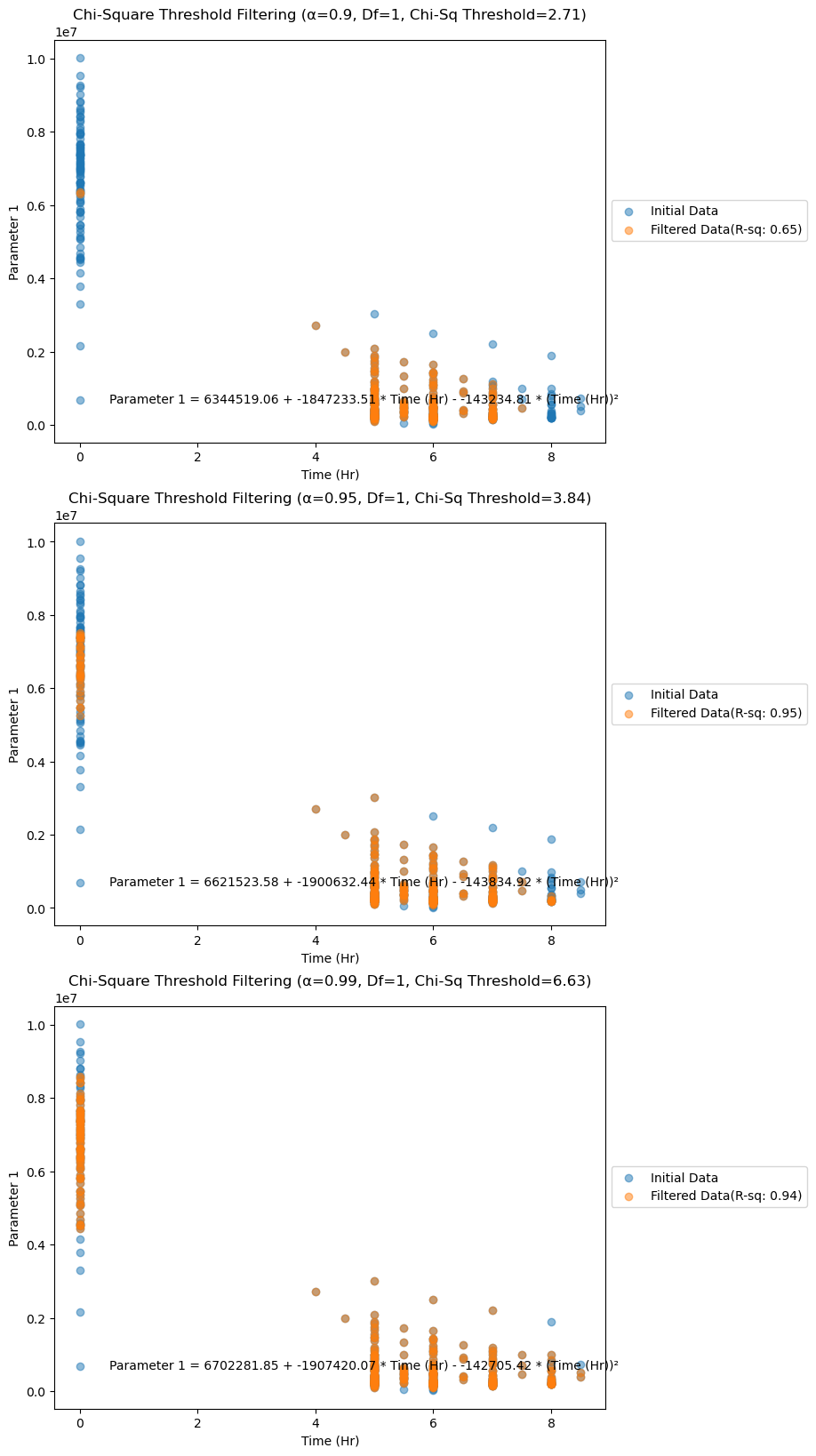
Figure 7. Filtered data (by Mahalanobis Distance analysis) plotted for Parameter 1.

Figure 8. Filtered data (by Mahalanobis Distance analysis) plotted for Parameter 2.
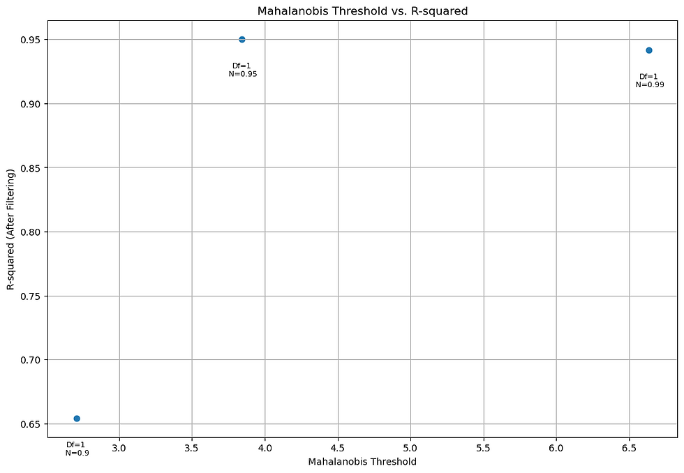
Figure 9. Chi-Squared Threshold vs R-Squared values for Parameter 1.
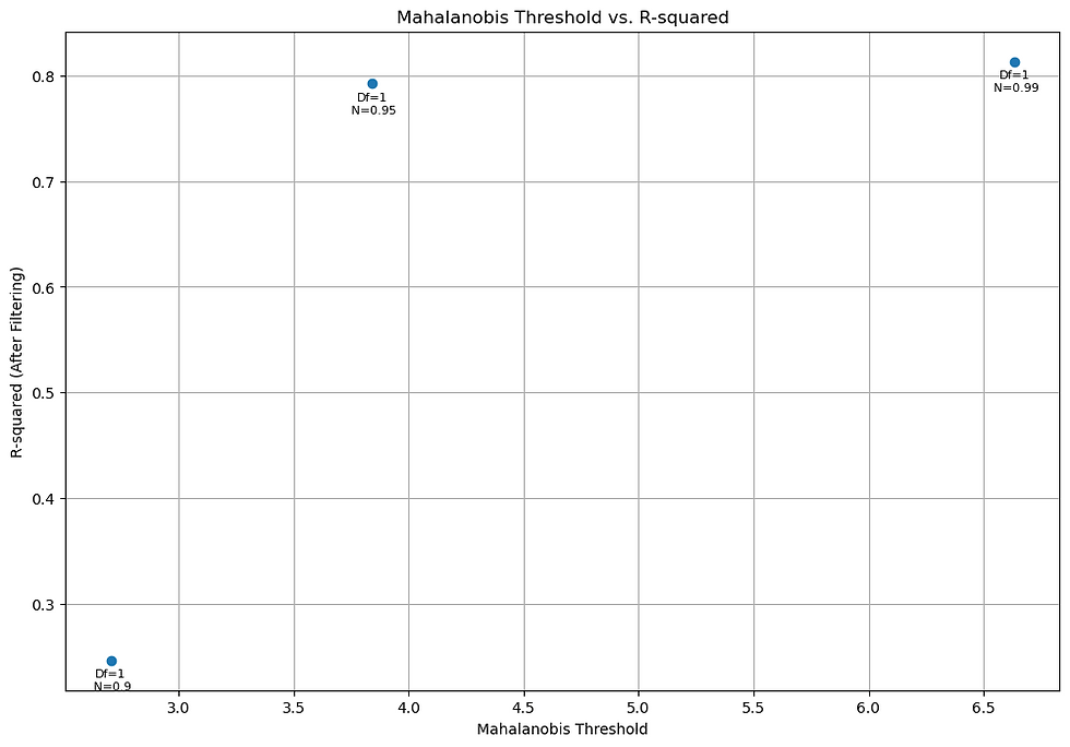
Figure 10. Chi-Squared Threshold vs R-Squared values for Parameter 2.
These filtering techniques significantly enhance the robustness of the model while preserving the fitted parameters. Adjusting the threshold values allows you to strike a balance between noise reduction and information retention, ultimately improving the reliability of your analysis.